
This example shows how you can set up a simple financial report in Excel using data from the Konnect Framework.
The report is based on two key elements:
- A structured dataset (from Konsolidator tables)
- Standard Excel formulas (SUMIFS and VLOOKUP)
By combining these, you can create a flexible report, such as a Profit & Loss statement.
Info box: Before you start
Open our Konnect Framework startup file here: *Link to article with the file*(you will find the newest version in the end of the article)
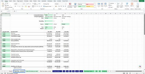
This file has a sheet called “Reporting – example”. In this article, we will go through this reporting example to help you understand how it is set up so you can continue and customize your own report.
When do you use the Konnect framework?
You typically use this setup when you want to:
- Build your own reports outside Konsolidator
- Compare scenarios (e.g. Actual vs Budget)
- Customize layout and presentation in Excel
- Reuse Konsolidator data in a familiar format
How it works
The report is built in three simple layers:
1. Header section (filters)
At the top of the sheet, you define the filters that control the report.
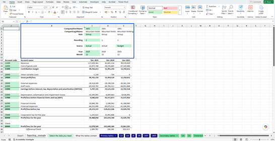
For example:
- Company
- Role (e.g. Group)
- Source (Actual, Budget, etc.)
- Year and Month
- Rounding
Each column uses these inputs, allowing you to show multiple scenarios side by side. For example, by comparing different years, months, or sources (Actuals vs Budget)
|
Cell |
Information |
|
C1 |
The company short name of the company you want to be reflected in your report. This should be from your company structure in Konsolidator. |
|
C3 |
The company role that should be reflected in the report, such as Group, Parent, or Contribution. |
|
C5 |
The rounding the is used to selected what to display the units in the report. |
|
C7 |
The source you want to be reflected in the report, such as Actual or Budget. |
|
C9 |
The year you want to be shown in the report. Enter the year in YYYY format. Consolidation must be completed in Konsolidator for the selected year before data is available. |
|
C10 |
The month you want to be shown in the report. Enter the month in M format. Consolidation must be completed in Konsolidator for the selected month before data is available. |
|
A13 |
A group account number that you know contains data. |
These are the “filters” used for the Amount in cell C13.
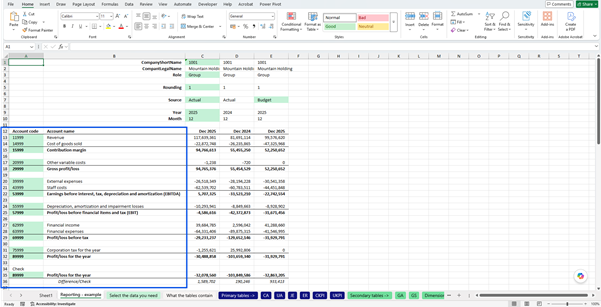
2. Report structure (rows)
The rows represent your reporting lines, for example:
- Revenue
- Costs
- EBITDA
- Profit/loss
Each row is linked to an Account Code, which is used to retrieve the data.
3. Data retrieval using formulas
This is the most important part of the setup.
Understanding the SUMIFS formula
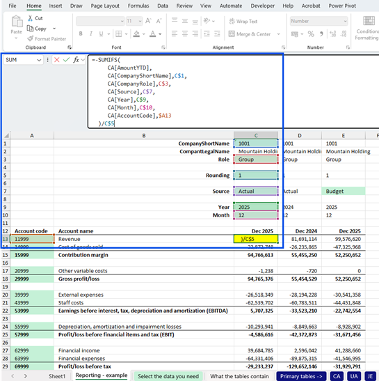
The SUMIFS formula is used to pull values from the Konsolidator dataset.
Example
=SUMIFS(
CA[AmountYTD];
CA[CompanyShortName];C$1;
CA[CompanyRole];C$3;
CA[Source];C$7;
CA[Year];C$9;
CA[Month];C$10;
CA[AccountCode];$A13
)/C$5
What the formula does
The formula sums values in the column called “AmountYTD” from the CA (Consolidated Accounts) table based on multiple conditions:
- Filters the selected CompanyShortName (in cell C1)
- Filters the selected CompanyRole (in cell C3)
- Filters by Source (Actual, Budget, etc.) (in cell C7)
- Filters by Year and Month (in cell C9 and C10)
- Filters the Account Code for the current row (in cell A13)
Finally, the result is divided by the rounding value (in cell C5).
If you would like to display the Amount in periodic figures you can change “AmountYTD” in the formula to “AmountPeriod”. Look at the CA table for the reference columns.
Why SUMIFS is important
SUMIFS is the engine of the report.
It ensures that:
- Data is always filtered correctly
- The report updates automatically when you change inputs
- You can reuse the same formula across all rows and columns and get different periods or sources by typing different information in the header filters.
Understanding the VLOOKUP formula
The VLOOKUP formula is used to retrieve the account names from the GA table.
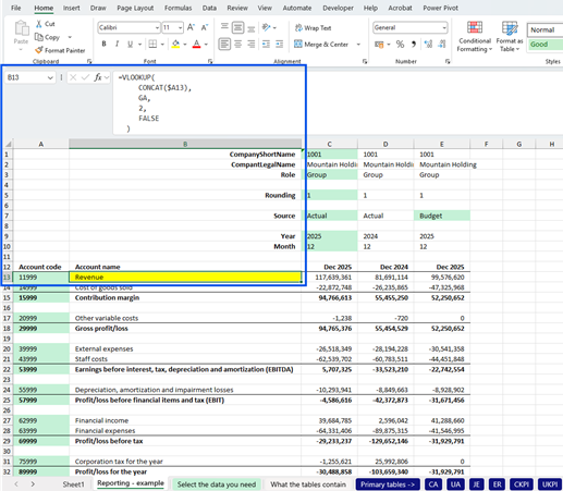
Example
=VLOOKUP(Concat($A13); GA; 2; FALSE)
What the VLOOK formula does
- Takes the Account Code from column A (cell A13 in this example)
- Looks it up in the GA (Group Accounts) table
- Returns the corresponding account name
Why VLOOKUP is useful
VLOOKUP ensures that:
- Your report uses consistent account names
- You avoid manually typing descriptions for account names
- The report stays aligned with Konsolidator’s account structure
Understanding the VLOOKUP formula
Use the same logic as in the example to expand and customize the report to your needs.
You can add more columns and use the header filters to select different companies, sources, periods, or scenarios.
You can also add more rows and enter the relevant Account Codes in column A to display the relevant accounts you need in your report.
Key principles
- The report is controlled by the header filters
- Each column represents a scenario (period, source, company)
- Each row represents an account code
- SUMIFS retrieves the numbers
- VLOOKUP retrieves the labels
Troubleshooting
If your report does not show expected values:
- Check that all filters (company, year, month, source) are correct
- Ensure the account code exists in the dataset
- Verify that the CA and GA tables are updated
- Check rounding if numbers seem too small or large
Support
If you need help, contact:
support@konsolidator.com